Why Finding “Nearby” Is Harder Than You Think—And How Geohashes Solve It
Searching for the closest coffee shop sounds simple, but geospatial queries are tricky. Learn how geohashes make location-based searches efficient and scalable.
Suppose you are building a location-based service like Yelp or DoorDash. A customer wants to find restaurants near them that match certain preferences. Their device provides a GPS location (latitude, longitude), and your app needs to quickly retrieve relevant restaurants in their vicinity.
But how do you efficiently query locations in a database? Traditional indexing methods, such as B-Trees, are optimized for sorting and searching one-dimensional data (e.g., numbers or strings). However, geographic locations exist in two dimensions, making proximity-based searches challenging.
A naive approach—scanning all locations and filtering those within a given radius—is inefficient at scale. To handle this, modern applications use geospatial indexes, which structure location data in a way that enables efficient retrieval of nearby points.
One such indexing method is geohashing, which encodes latitude and longitude into a compact, searchable format that allows for efficient range queries and neighbor lookups. In this article, we’ll explore how geohashing works, how to encode and decode locations, and how it is used in real-world applications like ride-sharing and food delivery services.
Understanding Geohashes: A Space-Efficient Way to Index Locations #
Geohashing is a method of encoding geographic coordinates (latitude and longitude) into a compact, hierarchical string representation. While the underlying principles date back to 1966 with G.M. Morton’s work on Z-order curves 1, the term “geohash” was popularized in 2008 by Gustavo Niemeyer2. Niemeyer’s implementation introduced Base32 encoding, allowing for shorter, human-readable representations of locations while maintaining spatial hierarchy.
For example, the geohash "sr2yk3c" precisely identifies the Colosseum in Rome, while a shorter geohash like "sr2y" covers most of Rome, and "sr" represents a broader region, including much of the Italian Peninsula. As you can see, each additional character in a geohash increases its precision by further subdividing the geographic area.
How Geohashing Works #
Geohashing transforms two-dimensional latitude and longitude coordinates into a one-dimensional string. This is done by recursively dividing the Earth’s surface into smaller and smaller grid cells.
- The world is initially divided into 4 rows and 8 columns, forming 32 cells.
- Each cell is assigned a character from a Base32 encoding set (
0123456789bcdefghjkmnpqrstuvwxyzi.e. all digits + all lowerchase characters excepta,l,i, ando). - Each of these 32 cells is further subdivided into another 32 smaller cells, continuing this pattern recursively.
- The resulting sequence of characters uniquely identifies a location, with longer geohashes representing finer precision.
This hierarchical structure enables geohashes to be used for efficient spatial indexing—shorter geohashes cover larger areas, while longer geohashes provide pinpoint accuracy.
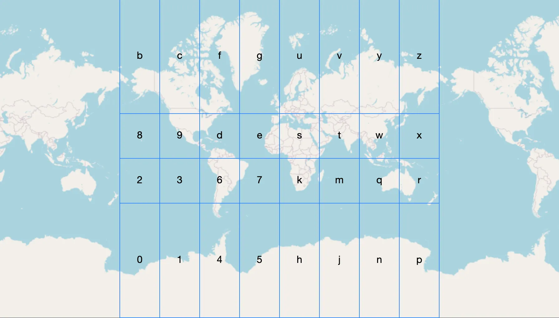
Fig 1. Entire world split into 32 top level geohash cells.
Advantages and Limitations of Geohashes #
Why Geohashing is Useful #
- Efficient proximity queries: Locations with similar geohashes are often spatially close, allowing for quick nearest-neighbor searches.
- Compact representation: A geohash string is typically shorter than storing raw latitude/longitude as floating-point values.
- Hierarchical properties: Shorter prefixes allow for easy region-based filtering.
- URL-friendly encoding: Since geohashes use Base32 encoding, they are URL-safe and human-readable.
Challenges and Limitations #
- Edge discontinuities: Adjacent locations near geohash boundaries may have vastly different geohash values, complicating neighbor searches.
- Geometric distortion: Since geohashes divide the world into a rectangular grid, they do not perfectly align with the Earth’s more spherical shape. This leads to varying cell sizes at different latitudes.
The Role of Space-Filling Curves in Geohashing #
Geohashing relies on Z-order curves (Morton curves) to map 2D coordinates into a 1D space while preserving spatial locality. (sidenote: Space filling curves are continuous lines that can pass through every single point in a higher dimensional space like a square or a cube. You can watch this youtube video from 3Blue1Brown to learn more about them. ) like the Z-curve are useful because they:
- Maintain spatial proximity, meaning nearby points in 2D space often remain close in 1D geohash representation.
- Enable fast neighbor computations, as neighboring geohashes can be determined using bitwise operations.
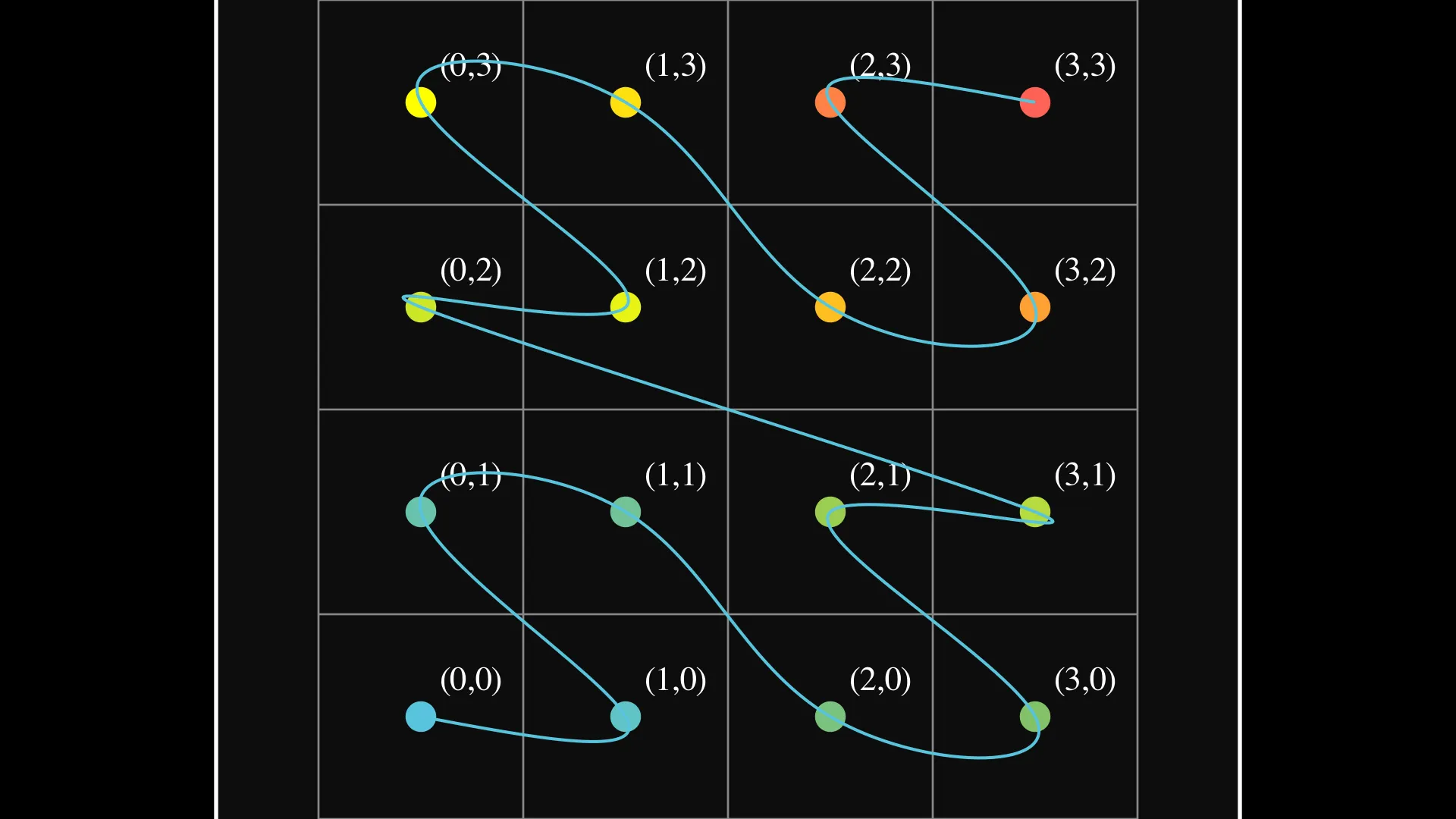
Fig 2. Z-Curve Space-Filling Pattern (4x4 Grid)
Points are visited in Z-shaped patterns at multiple scales, creating a space-filling curve that preserves locality
However, Z-curves are not perfect. Some cases require additional checks to ensure proper neighbor retrieval, especially at cell boundaries.
With this foundation, let’s now dive into how geohashing works in practice by encoding latitude and longitude into a geohash string.
Encoding Latitude and Longitude into a Geohash #
In the previous section, we explored why geohashes are useful. Their compact Base32 representation reduces storage footprint, and their hierarchical nature enables efficient proximity searches—critical for applications like Yelp, DoorDash, and Uber.
Now, let’s dive into how geohashes are created by encoding latitude and longitude into a short Base32 string.
Step-by-Step Encoding Process #
Step 1: Define Latitude & Longitude Ranges
Latitude and longitude define a point on the Earth’s surface:
- Latitude (horizontal lines) ranges from −90° to +90°, measuring distance north or south of the equator.
- Longitude (vertical lines) ranges from −180° to +180°, measuring distance east or west of the Prime Meridian.
For this walkthrough, we’ll encode the coordinates of Willis Tower in Chicago (41.878738, -87.6359612).
Step 2: Convert to Binary by Recursively Halving the Range
This step is similar to binary search—we iteratively halve the range and output
a 0 or 1 based on whether the value is in the lower or upper half.
Encoding Latitude (41.878738)
We start with range [-90, 90] and refine it bit by bit.
| Step | Midpoint | New Range | Bit |
|---|---|---|---|
| 1 | 0.0 | [0, 90] | 1 |
| 2 | 45.0 | [0, 45] | 0 |
| 3 | 22.5 | [22.5, 45] | 1 |
| 4 | 33.75 | [33.75, 45] | 1 |
| 5 | 39.375 | [39.375, 45] | 1 |
| 6 | 42.1875 | [39.375, 42.1875] | 0 |
| 7 | 40.78125 | [40.78125, 42.1875] | 1 |
| 8 | 41.484375 | [41.484375, 42.1875] | 1 |
| 9 | 41.8359375 | [41.8359375, 42.1875] | 1 |
| 10 | 42.01171875 | [41.8359375, 42.01171875] | 0 |
| 11 | 41.923828125 | [41.8359375, 41.923828125] | 0 |
| 12 | 41.8798828125 | [41.8359375, 41.8798828125] | 0 |
| 13 | 41.85791015625 | [41.85791015625, 41.8798828125] | 1 |
| 14 | 41.868896484375 | [41.868896484375, 41.8798828125] | 1 |
| 15 | 41.8743896484375 | [41.8743896484375, 41.8798828125] | 1 |
| 16 | 41.87713623046875 | [41.87713623046875, 41.8798828125] | 1 |
| 17 | 41.878509521484375 | [41.878509521484375, 41.8798828125] | 1 |
| 18 | 41.87919616699219 | [41.878509521484375, 41.87919616699219] | 0 |
| 19 | 41.87885284423828 | [41.878509521484375, 41.87885284423828] | 0 |
| 20 | 41.87868118286133 | [41.87868118286133, 41.87885284423828] | 1 |
Final Latitude Binary: 10111000101001101110
Encoding Longitude (-87.6359612)
We start with range [-180, 180] and refine it bit by bit.
| Step | Midpoint | New Range | Bit |
|---|---|---|---|
| 1 | 0.0 | [-180, 0] | 0 |
| 2 | -90.0 | [-90, 0] | 1 |
| 3 | -45.0 | [-90, -45] | 0 |
| 4 | -67.5 | [-90, -67.5] | 1 |
| 5 | -78.75 | [-90, -78.75] | 1 |
| 6 | -84.375 | [-90, -84.375] | 1 |
| 7 | -87.1875 | [-90, -87.1875] | 1 |
| 8 | -88.59375 | [-88.59375, -87.1875] | 0 |
| 9 | -87.890625 | [-88.59375, -87.1875] | 1 |
| 10 | -87.5390625 | [-87.890625, -87.1875] | 0 |
| 11 | -87.71484375 | [-87.890625, -87.71484375] | 1 |
| 12 | -87.802734375 | [-87.890625, -87.802734375] | 1 |
| 13 | -87.8466796875 | [-87.890625, -87.8466796875] | 1 |
| 14 | -87.86865234375 | [-87.890625, -87.86865234375] | 1 |
| 15 | -87.879638671875 | [-87.890625, -87.879638671875] | 1 |
| 16 | -87.8851318359375 | [-87.890625, -87.8851318359375] | 0 |
| 17 | -87.88238525390625 | [-87.8851318359375, -87.879638671875] | 0 |
| 18 | -87.88101196289062 | [-87.88238525390625, -87.879638671875] | 1 |
| 19 | -87.88032531738281 | [-87.88101196289062, -87.879638671875] | 1 |
| 20 | -87.8799819946289 | [-87.88032531738281, -87.879638671875] | 1 |
Final Longitude Binary: 01011110101111001111
Step 3: Interleave Bits
We now interleave the bits, alternating lat/lon.
| Lat Bits | 10111000101001101110 |
|---|---|
| Lon Bits | 01011110101111001111 |
Interleaved:11001101111000010110111001111011010111
Resulting 20-bit binary: 10011011110111101010
Step 4: Convert to Base32
Next, we split the 20-bit binary into 5-bit groups and convert each to a Base32 character:
Now, we convert every 5-bit chunk to Base32:
11001 10111 10000 10110 11100 11110 11010 111xx
Base32 Mapping:
11001→ d10111→ p10000→ 310110→ w11100→ j11110→ z
Final Base32 Geohash: Jorren Hendricks: https://geohash.jorren.nl/#dp3wjz"dp3wjz"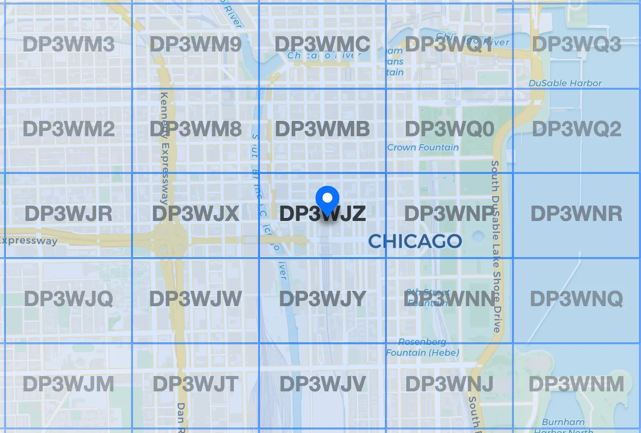
Fig 3. Geohash of the Willis Tower in Chicago
Python Implementation #
Now, let’s look at implemention of geohash encoding in Python. This is a
slightly simplified and non-optimized version.
class Geohash:
    BASE32 = "0123456789bcdefghjkmnpqrstuvwxyz"

    def __init__(self, precision=6):
        self.precision = precision  # Number of geohash characters

    def _latlon_bin(self, value: float, lo: float, hi: float, bit_length: int) -> str:
        """Convert latitude or longitude to a binary representation."""
        res = []
        for _ in range(bit_length):
            mid = (lo + hi) / 2
            if value > mid:
                lo = mid
                res.append('1')
            else:
                hi = mid
                res.append('0')
        return ''.join(res)

    def encode(self, lat: float, lon: float) -> str:
        """Encode a latitude and longitude into a geohash."""
        bit_length = self.precision * 5  # 5 bits per Base32 character

        # Get binary representation of latitude and longitude
        lat_bin = self._latlon_bin(lat, -90, 90, bit_length // 2)
        lon_bin = self._latlon_bin(lon, -180, 180, bit_length // 2)

        # Interleave latitude and longitude bits
        interleaved_bin = ''.join(
            lon_bin[i] + lat_bin[i] for i in range(len(lat_bin))
        )

        # Convert binary to Base32
        geohash = ''.join(
            self.BASE32[int(interleaved_bin[i:i+5], 2)]
            for i in range(0, len(interleaved_bin), 5)
        )

        return geohash

# Example Usage
geo = Geohash(precision=6)
encoded = geo.encode(41.878738, -87.6359612)  # Willis Tower
print(f"Encoded Geohash: {encoded}")
Summary of the Encoding Process #
- Recursively divide latitude and longitude into binary by checking if they fall above or below the midpoint.
- Interleave the bits, alternating longitude and latitude.
- Convert the binary sequence to Base32 to form the final geohash.
This process results in a short, hierarchical geohash that efficiently represents a geographic location.
With encoding covered, we now turn our attention to decoding geohashes back into latitude and longitude in the next section.
Decoding a Geohash #
In the encoding section, we transformed a latitude and longitude pair into a compact Base32 string. Now, we’ll reverse the process—converting a geohash back into latitude and longitude. Once you understand encoding, decoding becomes straightforward as it essentially follows the same steps in reverse.
Step-by-Step Decoding Process #
Step 1: Convert Base32 to Binary
- Each geohash character represents 5 bits.
- Convert each character back into its 5-bit binary equivalent.
- Example: If our geohash is “rffv”, we first convert it into a 20-bit binary string.
Step 2: Separate the Interleaved Bits
- Recall that encoding interleaves longitude and latitude bits.
- Now, we separate the even-indexed bits for longitude and odd-indexed bits for latitude.
Step 3: Reverse the Binary Search Process
- Start with the full latitude range
[-90, 90]and full longitude range[-180, 180]. - Iteratively refine the ranges using the separated bit sequences, just like encoding but in reverse.
- Each 1 means we take the upper half of the range, while each 0 means we take the lower half.
Step 4: Compute the Final Coordinates
- After processing all bits, we obtain a final range for both latitude and longitude.
- The final decoded latitude and longitude are the midpoints of their respective refined ranges.
Python Implementation #
We’ll implement a function that:
- Converts a geohash to its binary representation.
- Separates the interleaved bits for latitude and longitude.
- Performs a reverse binary search to refine coordinate ranges.
- Returns the midpoint of the final latitude and longitude ranges.
Example usage with "rffv" should return coordinates close to (41.878738, -87.6359612).
Summary of the Decoding Process #
- Convert Base32 geohash to binary.
- Separate latitude and longitude bit sequences.
- Iteratively refine coordinate ranges based on the binary values.
- The final decoded latitude and longitude are the midpoints of their respective final ranges.
Now that we can encode and decode geohashes, the next step is understanding how to find neighboring geohashes efficiently. This is crucial for location-based services like ride-sharing, food delivery, and geospatial databases.
Finding Nearest Neighbors in Geohash #
Location-based services frequently compute the nearest neighbors of a geohash to find nearby places, users, or points of interest. Understanding how this works under the hood is crucial for applications like geospatial databases, ride-sharing, and real-time location tracking.
Step-by-Step Process for Finding Neighbors #
Step 1: Decode to Find the Center of the Current Cell
- Use
decodeto obtain the latitude and longitude corresponding to the center of the geohash.
Step 2: Compute the Cell Size Based on Geohash Precision
- The size of a geohash cell (height and width) varies based on precision.
- Estimate the cell height (latitude span) and cell width (longitude span) based on the number of bits allocated to each.
Step 3: Compute the Coordinates for the 8 Neighboring Cells
- The 8 neighbors are in the N, S, E, W, NE, NW, SE, SW directions.
- Adjust latitude and longitude by the calculated cell height and cell width.
- Handle boundary conditions:
- Latitude bounds: Must stay within
[-90, 90]. - Longitude wrapping: If it exceeds
180, wrap it within[-180, 180].
- Latitude bounds: Must stay within
Step 4: Encode the New Locations Back to Geohashes
- Convert each of the computed neighbor coordinates back into geohash format with
encode.
Python Implementation #
def _get_cell_size(self, precision: int) -> tuple[float, float]:
    """Calculate the approximate size of a geohash cell for a given precision.

    Args:
        precision (int): precision/length of geohash

    Returns:
        (latitude_error, longitude_error)
    """
    lat_bits = precision * 5 // 2
    lon_bits = precision * 5 - lat_bits

    lat_err = 180.0 / (1 << lat_bits)
    lon_err = 360.0 / (1 << lon_bits)

    return lat_err, lon_err

def get_neighbors(self, geohash: str) -> dict[str, str]:
    """
    Compute the 8 neighboring geohashes (N, S, E, W, NE, NW, SE, SW).
    """
    center_lat, center_lon = self.decode(geohash)
    lat_height, lon_width = self._get_cell_size(len(geohash))
    directions = {
        "n": (lat_height, 0),
        "s": (-lat_height, 0),
        "e": (0, lon_width),
        "w": (0, -lon_width),
        "ne": (lat_height, lon_width),
        "se": (-lat_height, lon_width),
        "nw": (lat_height, -lon_width),
        "sw": (-lat_height, -lon_width),
    }
    neighbors = {}
    for direction, (dlat, dlon) in directions.items():
        nlat, nlon = center_lat + dlat, center_lon + dlon

        # handle latitude bounds
        nlat = max(min(nlat, 90), -90)

        # handle longitude wrapping
        if nlon > 180:
            nlon -= 360
        elif nlon < -180:
            nlon += 360

        neighbors[direction] = self.encode(nlat, nlon)
    return neighbors
Summary of finding the neighbors #
- Decode the geohash to find the center latitude and longitude.
- Compute the cell size for the given precision.
- Compute the neighboring coordinates by shifting latitude and longitude.
- Handle boundary conditions (latitude clamping, longitude wrapping).
- Encode the new coordinates back into geohashes.
Now that we can compute neighbors, let’s explore how this is used in geospatial databases.
Geohashes in Practice #
In the earlier sections, we explored encoding, decoding, and finding the nearest geohash neighbors of a given location. However, simply identifying neighboring geohash cells does not directly return the closest objects we seek. To achieve that, we need to query a geospatial database for all objects matching a geohash prefix and filter results based on actual proximity.
A common approach is to first check whether the current geohash cell contains enough points. The optimal geohash precision for such queries is typically 6 to 7 characters, balancing accuracy and coverage. If there aren’t enough points within this initial cell, we must expand the search space. This is usually done using a breadth-first search (BFS), exploring neighboring cells while ensuring each cell is visited only once. The search terminates as soon as a sufficient number of points are found—either stopping immediately if we only care about retrieving a minimum number of results or continuing until a full layer is processed for precise ordering.
Building such a system from scratch would require implementing efficient spatial indexing and search strategies. Fortunately, several databases natively support geohashes and provide optimized ways to store, index, and retrieve geospatial data. Two widely used systems that integrate geohashes are Redis and Elasticsearch.
Using Redis for Geospatial Queries #
Redis provides built-in support for geospatial indexing via its GEOADD and GEOSEARCH commands,
making it easy to store and retrieve locations efficiently.
Below, we demonstrate how a food delivery service could use Redis to manage restaurant locations.
Storing Locations in Redis
# GEOADD restaurants -73.9857 40.7484 "restaurant:1001"  # CLI equivalent
r.geoadd("restaurants", (lon, lat, restaurant_id))
Each entry consists of longitude, latitude, and a unique identifier, allowing us to store millions of locations efficiently.
Querying Nearby Locations
To find the closest restaurants for a given user location, we can use GEOSEARCH, which efficiently
retrieves nearby locations within a specified radius.
# Retrieving restaurants within 3 km of a customer
customer_id, customer_lat, customer_lon = customers[0]

res = r.geosearch(
    "restaurants",
    longitude=customer_lon,
    latitude=customer_lat,
    radius=3,
    unit="km",
    withdist=True,  # Include distances in the result
    sort="ASC",  # Sort results by proximity
)

print(f"Found {len(res)} restaurants near {customer_id}")
for rid, dist in res:
    metadata = r.hgetall(f"metadata:{rid}")
    print(f" - {metadata['name']} ({metadata['cuisine']}) - {dist:.2f} km away")
Optimized Querying: If a latitude-longitude pair is already stored in Redis
(e.g., user locations), we can use the member argument to directly perform the GEOSEARCH
query without manually providing coordinates.
Pagination with Redis #
In real-world applications, sending an unbounded list of search results to a client is inefficient.
Instead, pagination can be implemented using Redis Sorted Sets (ZSET). This allows storing query
results temporarily, sorted by distance, so that subsequent pages can be efficiently fetched.
def paginate_geosearch(
    key: str,
    lon: float,
    lat: float,
    radius: float,
    unit="km",
    page_size=5,
    page_num=1,
    session_id=None,
):
    if session_id is None:
        session_id = str(uuid.uuid4())

    temp_key = f"temp:{session_id}:key"

    if page_num == 1 and (not r.exists(temp_key) or r.ttl(temp_key) < 60):
        results = r.geosearch(
            "restaurants",
            longitude=lon,
            latitude=lat,
            radius=radius,
            unit=unit,
            withdist=True,
            count=MAX_INITIAL_RESULTS,
            sort="ASC",
        )
        pipe = r.pipeline()
        for member_id, distance in results:
            pipe.zadd(temp_key, {member_id: distance})

        pipe.expire(temp_key, 600)  # Set expiration for 10 mins
        pipe.execute()
    start = (page_num - 1) * page_size
    end = start + page_size - 1
    results = r.zrange(temp_key, start, end, withscores=True)
    return session_id, results
This method allows efficient paginated access to search results while ensuring that temporary data is cleaned up automatically using Redis’ Time-To-Live (TTL) feature.
Using Geohashes in Elasticsearch #
Elasticsearch provides powerful geospatial search capabilities
via its geo_point data type.
Unlike Redis, which primarily operates on simple radius-based lookups, Elasticsearch allows:
- Bounding box queries (find all objects within a rectangular area).
- Polygon-based queries (search within irregularly shaped regions).
- Distance-based ranking (sorting results by actual proximity).
Example: Storing & Querying Geohashes in Elasticsearch
To store a location in Elasticsearch, we can define a mapping with a geo_point field:
{
  "mappings": {
    "properties": {
      "location": { "type": "geo_point" }
    }
  }
}
We can then index a restaurant with a geohash:
{
  "name": "Pasta Place",
  "cuisine": "Italian",
  "location": {
    "lat": 40.7484,
    "lon": -73.9857
  }
}
To find restaurants within 3 km of a user’s location:
{
  "query": {
    "geo_distance": {
      "distance": "3km",
      "location": {
        "lat": 40.7484,
        "lon": -73.9857
      }
    }
  }
}
This allows scalable, full-text search with geospatial filters, making Elasticsearch ideal for applications that require complex queries, ranking, and filtering.
Apache Sedona: Geospatial Processing at Scale #
Apache Sedona is an open-source geospatial analytics library built on Apache Spark. Unlike Redis and Elasticsearch, which focus on real-time querying, Sedona is designed for large-scale geospatial data processing.
Who Uses Apache Sedona?
- Companies handling massive location datasets (e.g., satellite imagery, mobility analysis).
- Applications requiring spatial joins, clustering, and large-scale geospatial computations.
- Organizations leveraging big data frameworks (Spark, Hadoop) for spatial analysis.
Common Use Cases
- Ride-sharing & logistics: Computing optimal routes, identifying high-demand areas.
- Urban planning: Analyzing city-wide traffic patterns, infrastructure planning.
- Environmental monitoring: Processing satellite imagery to detect deforestation or pollution trends.
Apache Sedona supports geohashes for spatial partitioning and efficient indexing, making it valuable for big-data-driven geospatial applications.
Conclusion #
We explored how Redis and Elasticsearch provide built-in support for geospatial indexing using geohashes, each with different strengths:
- Redis is ideal for low-latency, real-time lookups with simple radius-based search.
- Elasticsearch is better suited for full-text search, ranking, and complex geospatial queries.
- Apache Sedona extends geospatial capabilities to big data processing at scale.
Next, we’ll look at what are some of the alternatives to geohashes.
Here’s a revised version of the alternatives section with clear, consistent details and a balanced view of advantages and disadvantages:
Geohash Alternatives in Geospatial Indexing #
While geohashes offer a compact and hierarchical way to index spatial data, they are not without limitations. Other spatial indexing methods have emerged, each with its own strengths and trade-offs. Below, we review three popular alternatives: R-Trees, S2Geometry, and H3.
R-Tree #
An R-Tree3 is a balanced tree structure designed to efficiently store spatial data by grouping objects using rectangular Minimum Bounding Regions (MBRs).
- Advantages:
- Efficient Nearest Neighbor Queries: Quickly finds all points within a specified rectangular area.
- Optimized for Window Queries: Excellent performance for range searches or “window” queries.
- Disadvantages:
- Dynamic Data Overhead: Insertion and deletion can be slightly slower, as the tree must be rebalanced.
R-Trees are widely used in spatial databases and systems such as PostGIS, MySQL, DuckDB and Elasticsearch.
S2Geometry #
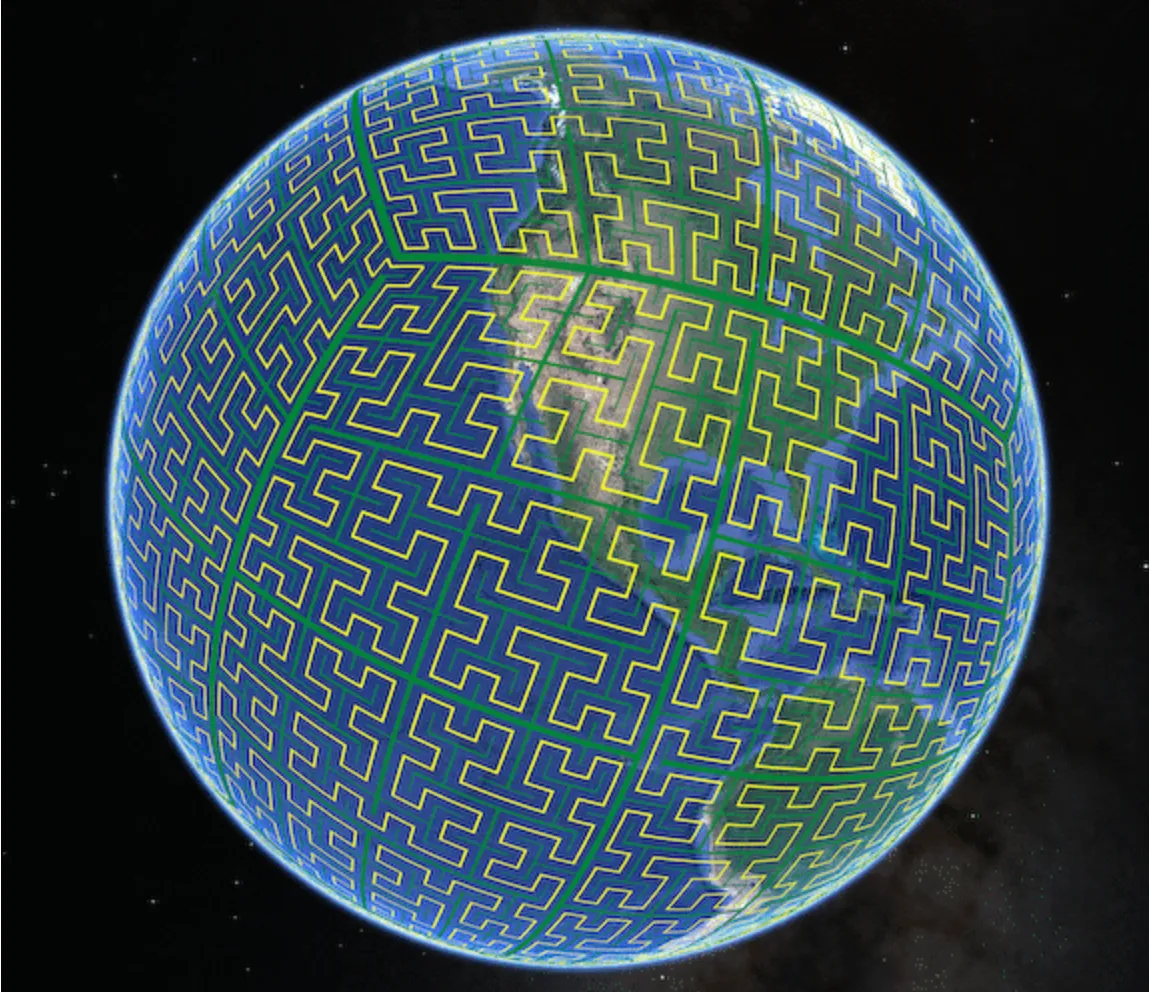
Fig 4. An illustration of the S2 curve after 5 levels of subdivision
S2Geometry: https://s2geometry.io
S2Geometry, developed by Google, uses a Hilbert space-filling curve to map the sphere into cells, providing a hierarchical spatial index.
- Advantages:
- Hierarchical Structure: Enables multi-level spatial queries and efficient indexing.
- Disadvantages:
- Moderate Distortion: Some distortion is introduced when mapping a spherical surface to a cell structure.
- Complex Implementation: The underlying algorithms can be complex to understand and implement.
S2Geometry is employed in systems like Google Spanner, CockroachDB, and DynamoDB’s geo library.
H3 #
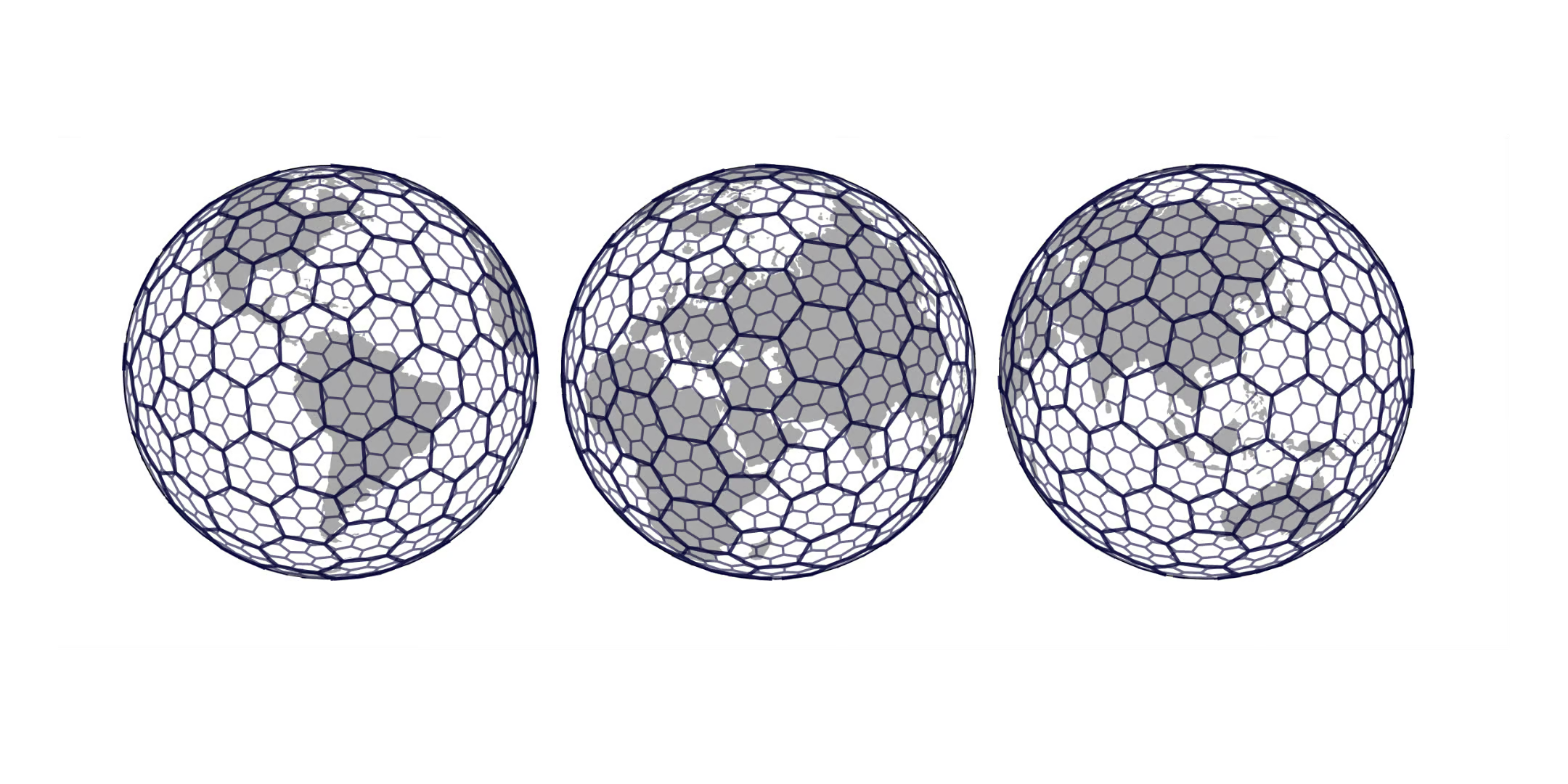
Fig 5. How Uber's H3 hierarchical spatial index allow users to partition the world into hexagons
Uber engineering blog https://www.uber.com/blog/h3/
H3, developed by Uber, is a hierarchical spatial index that uses hexagonal cells (with a few pentagons to cover the sphere) to represent geographic areas.
- Advantages:
- Low Distortion: Hexagonal cells provide more uniform coverage and equal distances between neighbors.
- Consistent Neighboring Distances: The geometry of hexagons ensures more consistent spatial relationships.
- Disadvantages:
- Complex Tiling: The hexagonal grid, especially with pentagonal adjustments, introduces complexity in indexing and computations.
H3 is popular for applications like ride pricing optimization, real-time geospatial analytics, and visualization.
Each of these alternatives offers a unique balance of performance, precision, and complexity. Choosing the right one depends on your specific application requirements, such as the nature of your queries, data update frequency, and the acceptable level of spatial distortion.
Closing Notes #
In this article, we explored geospatial indexing with a focus on geohashes—covering their encoding, decoding, neighbor lookups, and practical applications. We also discussed how databases like Redis and Elasticsearch efficiently leverage geohashes for spatial queries. Finally, we examined alternative geospatial indexing methods such as R-Trees, S2Geometry, and H3, each offering unique trade-offs in precision, query performance, and complexity.
Geohashes provide a compact and hierarchical way to index geospatial data, making them well-suited for many location-based applications. However, they are not a one-size-fits-all solution—depending on the use case, alternative indexing structures may offer better performance for nearest-neighbor searches, dynamic updates, or handling spherical distortions.
Understanding how these indexing methods work under the hood is crucial when designing geospatial systems that need to balance efficiency, accuracy, and scalability. Whether building a location-based search, a navigation system, or a geospatial analytics platform, choosing the right indexing approach will significantly impact performance and user experience.
With geospatial data playing a growing role in applications from ride-sharing to logistics and urban planning, mastering geohashes and their alternatives equips us with the tools to build more efficient and scalable systems.
You can find the full implementation of the geohash and my redis experiments in my github repo
Morton, G. M. (1966). “A Computer Oriented Geodetic Data Base and a New Technique in File Sequencing” (PDF). IBM Research. IBM Canada. Archived from the original on 2019-01-25. ↩︎
Niemeyer’s announcement “geohash.org is public!” of geohash can be seen at this archived page ↩︎
Guttmann, A. (1984). “R-Trees: A Dynamic Index structure for Spatial Searching” ↩︎