The Linked Hashmap Blueprint

For instance, consider a pharmacy like CVS or Walgreens, which uses patients’ Social Security Numbers (SSNs)—a nine-digit unique identifier—to manage patient information. Not all patients visit the pharmacy regularly, so it would be inefficient to store data in a large array indexed by SSNs. Instead, dictionaries allow us to store, retrieve, or delete patient information efficiently, even when the SSNs are sparsely distributed.

Building Blocks of a Hashmap #

To understand hashmaps, let’s break them down into their key components:

Hash Function #

A hash function is a mathematical transformation that maps an unbounded key space to a bounded one. This allows us to convert keys (e.g., SSNs) into indices within an array, which serves as the underlying storage for the hashmap.

For example, given a key \( k \), the hash function produces an index \( h(k) \) such that: \[ 0 \leq h(k) < \text{capacity of the hashmap} \]

More formally, a hash function can be described as: \[ h(x) \in \{ 0, 1, 2, \dots, m - 1 \}\; \text{for} \: x \in U \]

Here, \( m \) represents the size (capacity) of the hashmap, and \( U \) is the universe of possible keys.

However, this mapping introduces the challenge of hash collisions, where multiple keys may map to the same index. To ensure efficient performance, the choice of hash function and the collision resolution mechanism is critical.

Below, we explore two commonly used hashing strategies:

Division method #

The division method calculates the hash of a key \( k \) by taking the remainder when \( k \) is divided by a number \( m \): \[ h(k) = k \% m \]

Here, \( m \) is typically chosen as the size of the hashtable. Selecting \( m \) as a prime number reduces clustering and ensures better distribution of keys. Conversely, powers of 2 should generally be avoided for \( m \), as they can expose patterns in the data, breaking the randomness of the hash function.

Here’s a Python implementation of the division method:

def div_hash(k: int, m: int) -> int:
    return k % m

Multiplication method #

The multiplication method computes the hash of a key \( k \) by multiplying it with a constant \( A \) (where \( 0 < A < 1 \)), followed by scaling and flooring the result: \[ h(k) = \lfloor m \cdot (k \cdot A \mod 1) \rfloor \]

Unlike the division method, the multiplication method does not require \( m \) to be a prime number, making it more flexible. A commonly used value for \( A \) is approximately 0.618 (the golden ratio), which helps in achieving a good spread of keys.

Here’s a Python implementation of the multiplication method:

import math

def multiplication_hash(k: int, m: int, A: float = 0.61803398875) -> int:
    return math.floor(m * ((k * A) % 1))

Hash Collisions and Resolution #

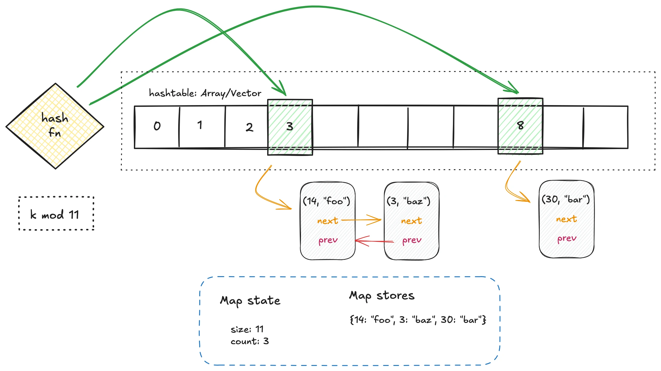
Hash collisions occur because the number of possible keys (the key space) is much larger than the bounded range of indices in the hashmap. In this implementation, collisions are resolved using chaining with a doubly linked list.

For optimal performance, it’s crucial for the hash function to produce a uniform distribution, ensuring keys are evenly spread across all buckets. This minimizes the risk of any single bucket being overloaded with collisions. A well-distributed hash function ensures that the average-case time complexity for get, put, delete, and contains operations remains \( O(1) \), even as the number of elements grows.

Why Use a Doubly Linked List? #

A doubly linked list enables \( O(1) \) insertion and deletion at arbitrary positions, making it ideal for efficient collision resolution when using chaining. Compared to alternatives like a singly linked list or dynamic arrays:

• A singly linked list would allow only \( O(1) \) insertion at the head but would require \( O(n) \) time for deletion at arbitrary positions.
• A dynamic array could handle collisions but would incur \( O(n) \) costs for resizing or inserting elements in the middle.

The doubly linked list strikes a balance, making it a natural choice for managing collisions efficiently.

Although this implementation uses chaining with a doubly linked list, alternative strategies such as open addressing with probing also exist. These strategies will be briefly discussed later in this article and explored in detail in a future piece. Resizing

To maintain efficiency as the hashmap grows, resizing is necessary. When the number of elements in the hashmap exceeds a certain threshold (determined by the load factor), the hashmap’s capacity is doubled, and all elements are rehashed to their new indices.

What is a Load Factor? #

The load factor threshold represents the ratio of the number of elements to the hashmap’s capacity. For example, a common threshold is 0.75, meaning a resize operation is triggered when 75% of the buckets are occupied. This threshold strikes a balance between space efficiency and performance, ensuring that buckets do not become overcrowded with collisions.

Here’s an example implementation of the resizing process:

def _resize(self):
    old_hashtable = self._hashtable
    self._size *= 2  # Double the capacity
    self._hashtable = [None] * self._size
    self._count = 0

    for dll in old_hashtable:
        if dll is not None:
            for node in dll:  # Reinsert elements into the new hashtable
                self.put(node.val[0], node.val[1])

Complexity: \( O(n) \), since every element must be rehashed and inserted into the new hashtable. Example Scenario:

Consider the following example of resizing:

• Original size: 23
• Key: 100
• Original hash: ( 100 % 23 = 8 )
• New size: 47
• New hash: ( 100 % 47 = 6 )

In this scenario, the hashmap doubles its size, and the key-value pairs are redistributed based on their new hashes. Resizing is computationally expensive ( O(n) ) because each element must be rehashed and reinserted. However, resizing is performed infrequently—only when the load factor exceeds the threshold—ensuring that the overall performance of the hashmap remains efficient.

Let’s explore the core operations and their implementation details:

Get and Contains Operations #

The get operation retrieves the value associated with a key, while contains checks whether a key exists in the hashmap. These operations rely on:

• Hashing the key to find the bucket.
• Traversing the linked list at the bucket to locate the key, if it exists.

Below is an implementation of the get and contains operations.

def get(self, key, default=None):
    idx = self._hash(key)
    self._validate_index(idx)
    dll = self._hashtable[idx]
    if dll == self._SENTINEL:
        return default
    for node in dll:
        if node.val[0] == key:
            return node.val[1]
    return default
    
def contains(self, key):
    """Check if key exists in dictionary."""
    idx = self._hash(key)
    self._validate_index(idx)
    dll = self._hashtable[idx]
    if dll == self._SENTINEL:
        return False
    for node in dll:
        if node.val[0] == key:
            return True
    return False

Complexity: \(O(1)\) on average, \(O(n)\) in the worst case (when all keys hash to the same bucket).

Put Operation #

The put operation inserts a new key-value pair or updates an existing key. Steps include:

• Calculating the hash for the key.
• Resolving any collisions by appending to or updating the linked list at the bucket.
• Resizing the hashmap if the load factor exceeds the threshold.

Below is an implementation of the put operation.

def put(self, key, value):
    idx = self._hash(key)
    self._validate_index(idx)
    if self._hashtable[idx] == self._SENTINEL:
        self._hashtable[idx] = DoublyLinkedList()
    dll = self._hashtable[idx]
    for node in dll:
        if node.val[0] == key:
            node.val = (key, value)
            return

    dll.append((key, value))
    self._count += 1

    # Resize if load factor exceeds 0.75
    if self._count / self._size > 0.75:
        self._resize()

Complexity: Similar to get — \(O(1)\) on average, \(O(n)\) in the worst case.

Delete Operation #

The delete operation removes a key-value pair. It involves:

• Hashing to locate the bucket.
• Removing the key from the linked list, which is efficient in \(O(1)\) due to the doubly linked list.

Below is an implementation of the delete operation.

def delete(self, key):
    idx = self._hash(key)
    self._validate_index(idx)
    dll = self._hashtable[idx]
    if dll == self._SENTINEL:
        raise KeyError(f"Key {key} not found")
    for node in dll:
        if node.val[0] == key:
            dll.delete_by_value(node.val)
            self._count -= 1
            return
    raise KeyError(f"Key {key} not found")

Complexity: Similar to get — \(O(1)\) on average, \(O(n)\) in the worst case.

Synchronized Linked Hashmap #

In concurrent environments, ensuring thread safety is critical. Here are two approaches to achieve synchronization:

• Naive Implementation Use a single lock for the entire hashmap. While simple, this approach severely limits concurrency since only one thread can access the hashmap at a time.
• Fine-Grained Locking Implement locks at the bucket level, allowing multiple threads to access different buckets concurrently. This improves throughput but increases implementation complexity.

Below is a partial implementation of a synchronized linked hashmap.

from threading import Lock

class FineGrainedLinkedHashTable(Dictionary):
    def __init__(self, size=23, hash_function=div_hash):
        self._size = size
        self._hashtable = [None] * self._size
        self._hash_function = hash_function
        self._locks = [Lock() for _ in range(self._size)]  # One lock per bucket

    def _hash(self, key):
        return self._hash_function(key, self._size)

    def get(self, key, default=None):
        idx = self._hash(key)
        with self._locks[idx]:
            dll = self._hashtable[idx]
            if dll is None:
                return default
            for node in dll:
                if node.val[0] == key:
                    return node.val[1]
            return default

Closing Notes #

Hashmaps are a fascinating data structure that balances simplicity and efficiency. The linked hashmap variant enhances functionality by maintaining order through a doubly linked list, making it suitable for use cases like LRU caches.

In this article, we focused on a chaining-based linked hashmap, complete with resizing and hash collision handling. In the future, we’ll explore open addressing with probing, comparing its trade-offs against chaining.

You can find the full implementation of the linked hash map in my github repo

References #

1. Algorithms lab youtube video